Ten great R functions #4
It is time again for some great R functions. The previous posts on great R functions can be found here, here, and here. As usual, some of these functions will not be of universal interest or relevance, but they are great when they are needed. Accordingly, this is more of a shout-out to functions I would like to recommend for specific use cases, and not examples of functions everybody should start using.
31. dplyr::filter_out()
Do you think about missing values when you use dplyr::filter()? Well, you should not miss out on that. This is one of the primary reasons why it is good to be familiar with the function filter_out() from {dplyr}. Let us begin with a simple example where we have a variable A in the data frame df with three values: 1, 2, and a missing value (NA). Here we can first use filter to explore what happens if we filter out all rows where A is different from 1.
df <- data.frame(A = c(1, 2, NA))

df |>
    dplyr::filter(A != 1)
#>   A
#> 1 2
You might be surprised to find out that a lot of mistakes in empirical work happen when people do not pay attention to what happens with missing data (especially with listwise deletion in regression analyses). So let us check out what happens when we use filter_out() to filter out rows where A is equal to 1.
df |>
    dplyr::filter_out(A == 1)
#>    A
#> 1 NA
#> 2  2
Here we see that the missing value is kept in our data frame. Accordingly, when using filter_out() we are being explicit about what exact rows we want to leave out rather than what rows we want to leave in. In other words, there are two ways to drop unnecessary rows from our data (keep what is necessary or delete what is not needed). As filter_out() was introduced in dplyr 1.2.0, it now gives you a good way to use filter() and filter_out() in line with what exactly you want to achieve with filtering your data. This is especially important when you are working with logical data (see this post for examples).
32. lemon::scale_x_symmetric()
There are many ways to visualise histograms, and especially when plotting standardised data, it is good to keep the axis symmetric to make it easy for the reader to interpret the distribution. One way to do this is to manually set the limits of the axis of interest (or automate it), but another easier way is to simply use scale_x_symmetric() from the {lemon} package. Here is a simple example where we plot the same data without and with lemon::scale_x_symmetric():
library("ggplot2")
library("patchwork")

figA <- airquality |>
    tidyr::drop_na(Ozone) |>
    ggplot(aes(Ozone - mean(Ozone))) +
    geom_histogram() +
    labs(title = "geom_histogram()")

figB <- airquality |>
    tidyr::drop_na(Ozone) |>
    ggplot(aes(Ozone - mean(Ozone))) +
    geom_histogram() +
    lemon::scale_x_symmetric() +
    labs(title = "+ lemon::scale_x_symmetric()")

figA + figB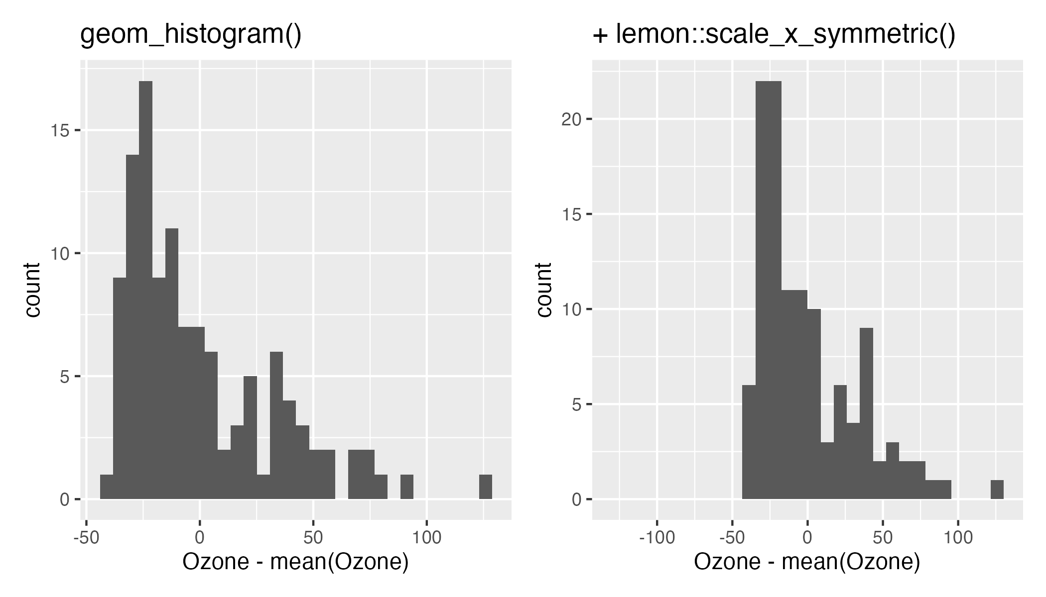
This makes it easier to see how exactly the data is distributed. I was not familiar with this function until I read this post by Nicola Rennie with recommendations for great ggplot2 functions. Do check it out.
33. dplyr::c_across()
If you need to perform row-wise aggregations across multiple columns, dplyr::c_across() in combination with dplyr::rowwise() is much easier than using base::c(). This is especially useful if you have tens or hundreds of columns you need to aggregate, but for the sake of simplicity and illustration, let us find the row-wise sum across three columns:
df <- data.frame(A = 1:3, B = 4:6, C = 7:9)

df |>
    dplyr::rowwise() |>
    dplyr::mutate(total = sum(dplyr::c_across(A:C)))
#> # A tibble: 3 × 4
#> # Rowwise:
#>       A     B     C total
#>   <int> <int> <int> <int>
#> 1     1     4     7    12
#> 2     2     5     8    15
#> 3     3     6     9    18
Again, this example might not look like much, but that is the beauty of it when you find yourself in a situation where you really need to perform row-wise aggregations.
34. janitor::tabyl()
I have recommended functions from the {janitor} package in the past, and it deserves another mention for the tabyl() function. The function is great at generating frequency tables for one or more columns. Here is a simple example on how to provide a frequency table for a single vector:
janitor::tabyl(mtcars$gear)
#>  mtcars$gear  n percent
#>            3 15 0.46875
#>            4 12 0.37500
#>            5  5 0.15625
We could of course rely on prop.table() to get the proportions, but janitor::tabyl() provides an easy and good overview without having to rely on multiple functions to get the proportions.
Another good example is how missing values are treated. Let us compare the function with table() on the same vector:
x <- sample(c(1:10, NA), 1000, replace = TRUE)

table(x)
#> x
#>   1   2   3   4   5   6   7   8   9  10
#>  98 106  97  83  82  90  80  93  87  93

janitor::tabyl(x)
#>   x   n percent valid_percent
#>   1  98   0.098    0.10781078
#>   2 106   0.106    0.11661166
#>   3  97   0.097    0.10671067
#>   4  83   0.083    0.09130913
#>   5  82   0.082    0.09020902
#>   6  90   0.090    0.09900990
#>   7  80   0.080    0.08800880
#>   8  93   0.093    0.10231023
#>   9  87   0.087    0.09570957
#>  10  93   0.093    0.10231023
#>  NA  91   0.091            NA
Notice how table() ignores NAs (unless explicitly specified with the useNA argument), and how janitor::tabyl() shows the percentage with and without the missing values included. For a lot more examples on how to leverage the function, check out the associated vignette.
35. lubridate::floor_date()
If you are working with dates and have to round the date (or even time), {lubridate} offers a lot of options with the functions round_date(), floor_date(), and ceiling_date(). In the example below we have a vector with dates and we want to round each date to the first of the month (using lubridate::floor_date() with the unit argument).
lubridate::floor_date(as.Date(c("2026-08-05", "2026-09-30", "2026-12-24")),
                      unit = "month")
#> [1] "2026-08-01" "2026-09-01" "2026-12-01"
It is not much but it is reliable and on time.
36. ggtranslate::ggtranslate()
I was recently working on a project where I had to provide the same ggplot2 objects in multiple languages. I found the package ggtranslate which was very useful for the purpose. I would call it underrated as it currently has zero stars on GitHub. What is great about the function is that it takes two inputs: a ggplot2 object and a list with translations. So you do not need to set up the same plot twice, and you only need to make changes to one plot and make sure that you provide the exact translations.
In the example below (modified from the example in the repo for the package), I create a simple plot in English, then I save the translations for the relevant labels in an object called dict_da, and then use ggtranslate::ggtranslate() to translate the plot to Danish. Finally, I show the English plot and the Danish plot next to each other.
library("ggplot2")
library("patchwork")

df <- data.frame(day = c("Monday", "Tuesday", "Wednesday",
                         "Thursday", "Friday", "Saturday"),
                 value = c(10, 12, 8, 11, 9, 12))

p_en <- ggplot(df, aes(y = value, x = day, fill = day)) +
    geom_col() +
    labs(title = "Weekly Report (English)",
         subtitle = "Sales data for the week",
         x = NULL,
         y = "Sales (in millions)") +
    theme(legend.position = "none") +
    coord_flip()

dict_da <- list("Weekly Report (English)" = "Ugentlig rapport (dansk)",
                "Sales data for the week" = "Salgsdata for ugen",
                "Sales (in millions)" = "Salg (i millioner)",
                "Monday" = "Mandag",
                "Tuesday" = "Tirsdag",
                "Wednesday" = "Onsdag",
                "Thursday" = "Torsdag",
                "Friday" = "Fredag",
                "Saturday" = "Lørdag")

p_da <- p_en |> ggtranslate::ggtranslate(dict_da)

p_en + p_da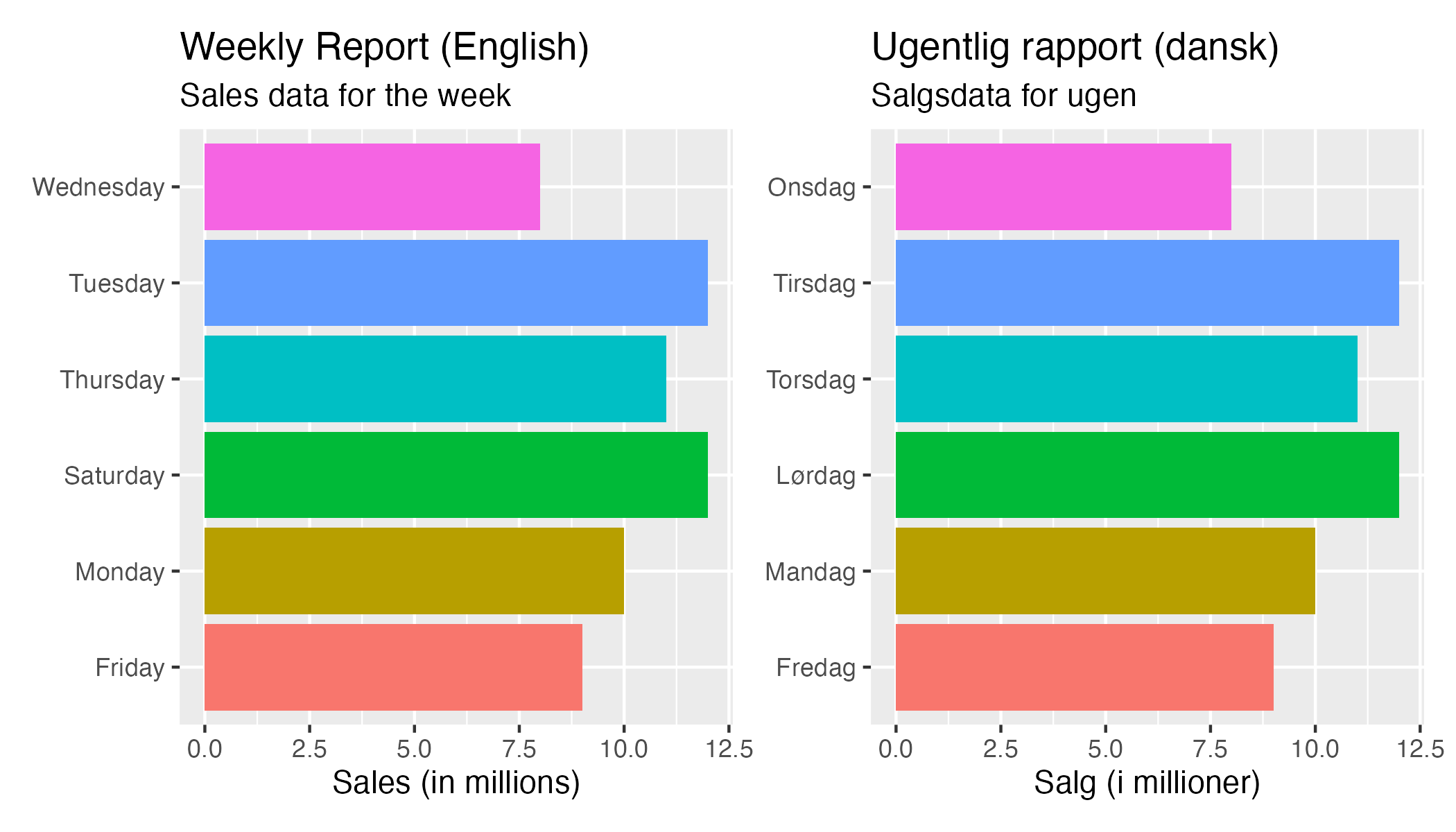
The two plots are identical with the only exception being the translations of the labels.
37. readr::cols()
If you use readr::read_csv() to load a CSV file into R, it will in most cases work without any issues, especially if your CSV file is well-structured. The function is good at understanding what data is available and assigning it to its correct data type. However, it is better to be explicit about what data you expect than rely on guessing.
Below is an example where we read 1,600 opinion polls for two parties (party_a and party_q). As party_q did not exist back in 2010 and this is where our dataset begins, the data is missing for a lot of rows. Notice here how the data is being imported as logical data (as the first 1000 rows are missing).
readr::read_csv("polls.csv")
#> Rows: 1600 Columns: 6
#> ── Column specification ────────────────────────────────────────────────────────
#> Delimiter: ","
#> chr (1): pollingfirm
#> dbl (4): year, month, day, party_a
#> lgl (1): party_q
#>
#> ℹ Use `spec()` to retrieve the full column specification for this data.
#> ℹ Specify the column types or set `show_col_types = FALSE` to quiet this message.
#> # A tibble: 1,600 × 6
#>    pollingfirm  year month   day party_a party_q
#>    <chr>       <dbl> <dbl> <dbl>   <dbl> <lgl>
#>  1 Gallup       2010     1    29    25   NA
#>  2 Greens       2010     2     3    26.2 NA
#>  3 Rambøll      2010     2    11    26.6 NA
#>  4 Gallup       2010     2    26    26.6 NA
#>  5 Greens       2010     3     3    28.4 NA
#>  6 Rambøll      2010     3     4    24.6 NA
#>  7 Gallup       2010     3    26    26.7 NA
#>  8 Rambøll      2010     3    30    27.4 NA
#>  9 YouGov       2010     4    12    28.1 NA
#> 10 Greens       2010     4    14    28.5 NA
#> # ℹ 1,590 more rows
Importantly, readr::read_csv() does not return an error and it will not stop you from using the party_q column. Let us look at the data where we have non-missing values. Here we see that we get 15 rows of data. These 15 rows of data are the cases where party_q is either 0.0 (FALSE) or 1.0 (TRUE) in the data.
readr::read_csv("polls.csv") |>
    na.omit()
#> Rows: 1600 Columns: 6
#> ── Column specification ────────────────────────────────────────────────────────
#> Delimiter: ","
#> chr (1): pollingfirm
#> dbl (4): year, month, day, party_a
#> lgl (1): party_q
#>
#> ℹ Use `spec()` to retrieve the full column specification for this data.
#> ℹ Specify the column types or set `show_col_types = FALSE` to quiet this message.
#> # A tibble: 15 × 6
#>    pollingfirm  year month   day party_a party_q
#>    <chr>       <dbl> <dbl> <dbl>   <dbl> <lgl>
#>  1 Voxmeter     2021    11    21    25.8 FALSE
#>  2 Voxmeter     2021    12     5    25.7 FALSE
#>  3 Voxmeter     2021    12    19    25.9 FALSE
#>  4 YouGov       2021    11     9    28   TRUE
#>  5 Voxmeter     2022     1    30    24.9 FALSE
#>  6 Voxmeter     2022     2    20    25.2 FALSE
#>  7 Voxmeter     2022     3    12    27   FALSE
#>  8 YouGov       2022     4    11    29.2 TRUE
#>  9 Epinion      2022     9    20    25.4 TRUE
#> 10 Voxmeter     2022    11    13    30   FALSE
#> 11 Voxmeter     2023     2     5    22.1 FALSE
#> 12 Epinion      2023     8    23    22.9 FALSE
#> 13 Epinion      2023    11    15    18.2 FALSE
#> 14 Epinion      2023    12    13    19.6 FALSE
#> 15 Verian       2024     3    21    20   TRUE
To avoid this, we can use the readr::cols() function to type what data we are expecting from the data we import. I will make an exception here and not actually show readr::cols() in action, but feel free to deep dive into the documentation on how it is used to create column specification. Instead, all you basically need to know is the compact string representation and the col_types argument when importing the data. In the example below I specify what type of data I want each column to be imported as. Again, I keep only the rows where we actually have data for party_q.
readr::read_csv("polls.csv", col_types = c("pollingfirm" = "c",
                                           "year" = "d",
                                           "month" = "d",
                                           "day" = "d",
                                           "party_a" = "d",
                                           "party_q" = "d")) |>
    na.omit()
#> # A tibble: 136 × 6
#>    pollingfirm  year month   day party_a party_q
#>    <chr>       <dbl> <dbl> <dbl>   <dbl>   <dbl>
#>  1 Voxmeter     2021    11    14    26.5     0.2
#>  2 Voxmeter     2021    11    21    25.8     0
#>  3 Voxmeter     2021    11    28    26       0.4
#>  4 Voxmeter     2021    12     5    25.7     0
#>  5 Epinion      2021    12     8    26.3     0.6
#>  6 Voxmeter     2021    12    11    24.3     0.1
#>  7 Gallup       2021    12     9    26.7     0.2
#>  8 Voxmeter     2021    12    19    25.9     0
#>  9 YouGov       2021    11     9    28       1
#> 10 YouGov       2021    12     6    29.3     0.9
#> # ℹ 126 more rows
Now we see that the columns are imported as expected. Accordingly, do not let the function try to guess what the data is. Be explicit. For the compact string representation, you can specify character (c), integer (i), number (n), double (d), logical (l), factor (f), date (D), date time (T), and time (t).
38. modelr::rmse()
I try not to recommend functions in packages that have not been updated for a long time, and while the {modelr} package has not been updated for years, it is still a stable and great package for model quality metrics.
So if we want to get the root-mean-squared-error (RMSE) of a model, we can use modelr::rmse() and specify the model and the data:
modelr::rmse(lm(mpg ~ wt, data = mtcars), mtcars)
#> [1] 2.949163
Other good functions in the package are mae() (mean absolute error) and qae() (quantiles of absolute error).
39. cmdstanr::install_cmdstan()
I was running a series of Bayesian hierarchical regression models using brms::brm(), but it took a long time to run the models in production. The package {cmdstanr} turned out to be very helpful, and I will recommend using cmdstanr when fitting Bayesian regression models. Here are the commands I included in my Dockerfile to install CmdStan via {cmdstanr}:
RUN R -e "install.packages('cmdstanr', repos = c('https://stan-dev.r-universe.dev', getOption('repos')))"
RUN R -e "cmdstanr::install_cmdstan()"
This will now make it possible to use 'cmdstanr' as the backend when fitting the Bayesian regression model with brms::brm().
brms::brm(..., backend = "cmdstanr")You will now be using a better compilation workflow with faster sampling and, accordingly, be able to run these regression models much faster.
40. cranlogs::cran_downloads()
The package {cranlogs} is great when you want to download logs from the RStudio CRAN mirror. I have used this package for a few different projects, including in my post on the most popular ggplot2 packages.
The function cranlogs::cran_downloads is intuitive to use and you do not need to rely on an API key or anything. Just use the function and you get the data. Here is an example where we get the number of downloads of the {ggplot2} package over the past week:
cranlogs::cran_downloads(when = "last-week",
                         package = "ggplot2")
#>         date count package
#> 1 2026-09-04 64306 ggplot2
#> 2 2026-09-05 47941 ggplot2
#> 3 2026-09-06 47721 ggplot2
#> 4 2026-09-07 69330 ggplot2
#> 5 2026-09-08 81050 ggplot2
#> 6 2026-09-09 88591 ggplot2
#> 7 2026-09-10 77523 ggplot2
Here we see that the {ggplot2} package was downloaded 77,523 times from the RStudio CRAN mirror on September 10.